Neural Networks on the Arduino Part 6: Putting it all together, training and testing your neural network

We are almost there! We can nearly put all the code together. All we need is some test data to call UpdateWeights with (for the training) and some test data (for the testing).

At this point it would be a good idea copy the source code into the Arduino IDE and follow this article while looking at the sources.

For one of the tests I'm going to use the same one as I used here in the Python implementation by Tariq Rashid. The neural network is presented with a spike in a graph and must return the position of that spike.

Here is how I create the test data:

// This creates a test input vector and the ideal output for that input
void CreatePositionTrainingSample (mtx_type* TrainInputVector,
                                   mtx_type* TrainTargetVector)
{
    // A check to stop silly errors as you meddle with the code...
    if (NUM_OUTPUTS != 2) {
        Serial.print ("Training sample error, I want 2 outputs!") ;
    }
 
    // Choose a place from 0 to (NUM_INPUTS-1)
    int iPos = random (0,NUM_INPUTS) ;  
   
    // Make a vector with a spike at the randomly chosen iPos
    for (int i = 0 ; i < NUM_INPUTS ; i++) {
        if (i == iPos) {
            TrainInputVector[i] = 1.0 ;      
        } else {
            TrainInputVector[i] = 0.0 ;
        }
    }
    // Now we have an input vector with a single non zero value

    // What is the expected output number?
    // We want one output to be at the "value of the position" so to speak
    double OutputValue1 = (double)iPos/double(NUM_INPUTS-1) ;

    // Just to have more than one output...
    // ...make other output to be at the "opposite of the value of the position"
    double OutputValue2 = 1.0 - OutputValue1 ;

    // This is the idea correct answer...
    TrainTargetVector[0] = OutputValue1 ;
    TrainTargetVector[1] = OutputValue2 ;
}

So if the function creates an input vector with a spike in the middle:

{0,0,1,0,0}  

I get an output value of 0.5.

And if the function creates an input vector with a spike at the end of the vector.

{0,0,0,0,1}  

I get an output vector 1.0.

And so on.


Actually, to keep things interesting, I have two outputs, the position of the spike and its mirror image, that is what OutputValue2 is in the above function.

Be careful with the use of random(). The second parameter is exclusive.

That position test is actually a simple problem for neural networks, a harder one is XOR. The XOR problem is what prompted the use of the hidden layer. The XOR problem cannot be solved with a single layer neural network. There's plenty on the internet about the XOR problem so I won't go into it here, but to make sure we've got things right in our two layer Arduino neural network we must test it with the XOR problem.

Basically if there are two inputs when both are active (=1) the output should be inactive (0). And if only one of the two inputs are active then the output should be active.

Looking at it another way, the neural network should detect if the two inputs are different. If they are both 0 or both 1 then the output should be 0.

Here's a table which illustrates that:


inputs       XOR    XNOR
0    0        0      1
0    1        1      0
1    0        1      0
1    1        0      1



I've added XNOR an output as well, just to make it interesting. XNOR is simply the opposite of XOR, as you can see in the above table.

Here's how I create a sample for the XOR training and testing:

void CreateXORTrainingSample (mtx_type* TrainInputVector, mtx_type* TrainTargetVector)
{
    // A check to stop silly errors as you meddle with the code...
    if (NUM_OUTPUTS != 2) {
        Serial.print ("Training sample error, I want 2 outputs!") ;
    }
    if (NUM_INPUTS != 2) {
        Serial.print ("Training sample error, I want 2 inputs!") ;
    }
    
    // Choose a row in the truth table...
    int iWhichRow = random (0,4) ;  // will give me a number from 0 to 3 inclusive

    if (iWhichRow == 0) {
        TrainInputVector[0] = 0 ;  // INPUT 1   
        TrainInputVector[1] = 0 ;  // INPUT 2
        TrainTargetVector[0] = 0 ; // XOR  
        TrainTargetVector[1] = 1 ; // XNOR  
       
    } else if (iWhichRow == 1) {
        TrainInputVector[0] = 1 ;     
        TrainInputVector[1] = 0 ;     
        TrainTargetVector[0] = 1 ;  
        TrainTargetVector[1] = 0 ;  

    } else if (iWhichRow == 2) {
        TrainInputVector[0] = 0 ;     
        TrainInputVector[1] = 1 ;     
        TrainTargetVector[0] = 1 ;  
        TrainTargetVector[1] = 0 ;  
   
    } else {
        TrainInputVector[0] = 1 ;     
        TrainInputVector[1] = 1 ;     
        TrainTargetVector[0] = 0 ;  
        TrainTargetVector[1] = 1 ;  
    }
}

Now, in the whole source code I've made it possible for you to use either of these tests by simply setting a define to 1:

// To decide the type of test one of these should be 1 and the other 0
#define XOR_TEST 0
#define POSITION_TEST 1


The number of inputs outputs and hidden nodes will change according to what sort of test you use.

Note also that in the same place in the code I set the  NUM_TRAINING_SAMPLES to depend on if we are doing XOR_TEST or POSITION_TEST. NUM_TRAINING_SAMPLES is much higher for the XOR test because XOR is a harder problem.

The top level of the program starts at void loop() near the end of the sources. First the network is trained, and then it is tested.

You need to run the serial monitor to see the output of the training and of the testing. Here is the output when POSITION_TEST is used:

TrainOnOneSample is called repeatedly (from inside RunMultipleTrain) in order to slowly modify the weights.

Inside TrainOnOneSample is the define QUERY_AS_YOU_UPDATE. If that is set to 1 then you will test the neural network after every single train and print the results. If it is set to 0 you will only see the final test results.

Now it is up to you to decide what...

1. light inputs
2. light outputs
3. motors
4. servos
5. solenoids
6. switches
7. relays
8. varistors
9. transistors
10. robots
11. robot arms
12. robot legs
13. touch sensors
14. pressure sensors
15. meteorological sensors
16. ...

...you want to use this program with!

Whatever you decide I think you'll probably need to increase the number of hidden nodes.

Part 7 the complete source code to a neural network on the Arduino

Neural Networks on the Arduino Part 4: Calculation of hidden errors in a neural network

Of all the things I found hard to "believe" "understand" or "grok" was how the hidden errors are calculated in a neural network. If you've done matrix maths the equation seems far too simple to be true. Here I'll illustrate to you, and to myself, how it works.

The problem is that while it is clear what an error is at the output of a neural network, it is not immediately clear what an error is at the hidden layer output. Graphically:

It turns out that a good approach is to use the errors at the output to set the "errors" in the hidden layer.

(By the way you can't just copy the output errors into the hidden layer because there is no guarantee that the number of outputs is the same as the number of hidden nodes. Plus the fact that you'd be arbitrarily jumping over the HiddenToOutput matrix.)

So the idea is that the hidden layer errors are weighted averages of the errors at the output. We make the assumption that an error at the output has been caused by an "error" in the hidden layer. How much the error at the output has been caused by the error in the hidden depends on the weight connecting the two nodes (errors).

For example look at eH2 above, it contributed to errors at eO1 and eO2, and how much it contributed depended on the weights wa and wb. So eH2 will be a weighted average of eO1 and eO2. As explained in the book by Tariq Rashid, we do not need to use an actual weighted average, we can just use the weights directly.

In other words...

eH2 = wa*eO1 + wb*eO2

Luckily this can be nicely done with matrices, and the matrix of the weights for this back propagation of errors is easily created from the forward hidden to output matrix.

I'm about to demonstrate that, by the magic of matrices, the matrix which gives us the hidden "errors" from the output errors is simply the transpose of the forward hidden to output matrix! Lets look again at how the forward hidden to output matrix works:

I've arranged the weights closer to the output nodes so you can see the calculation better. Study and understand how o1 is calculated. Compare the drawing and the matrix versions in the above image.

So. That is how the forward calculation of the outputs work. How do we do the backward propagation of the errors using matrix multiplication? Here's another, this time illustrating the backward propagation of errors from the output to the hidden layer:

• I've drawn the errors flowing rightwards, from eo1 to eh1 etc. This is so you can easily relate the diagram to the matrix multiplication.
• The o in eo2 (for example) stands for output
• The h in eh3 (for example) stands for hidden
• I've drawn the weights which modify the output errors to form the hidden "errors" close to the hidden error nodes
• I've drawn the hidden error calculations at top right of the image.
• I've drawn the matrix multiplication version in the bottom half.
• To be sure the weights have the correct indices try checking the weight which connects o1(eo1) to  h2(eh2) in both diagrams. In both diagrams it is w21.
• Note that the matrix in this diagram is the transpose of the matrix in the previous diagram.

E voila! That is why and how the transpose of the final forward matrix can be used to "invent" the hidden "errors" from the output errors.

Part 5 How To Update The Weights

Neural Networks on the Arduino Part 3: Details and tests of the matrix multiplication

(Read these Part 1 and Part 2 before reading this page)

Since I'm interested in getting all the neural network running on the Arduino and since neural networks use matrices, it is natural for me to use the MatrixMath.cpp library written for the Arduino by Charlie Matlack.

There was one thing I was not sure about though, can I use Matrix.Multiply function with vectors? I.e not just fully blown matrices with more than one row and more than one column. Maybe a silly question, but there your go.

I looked at the code for multiply:

//Matrix Multiplication Routine
// C = A*B
void MatrixMath::Multiply(mtx_type* A, mtx_type* B, int m, int p, int n, mtx_type* C)
{
    // A = input matrix (m x p)
    // B = input matrix (p x n)
    // m = number of rows in A
    // p = number of columns in A = number of rows in B
    // n = number of columns in B
    // C = output matrix = A*B (m x n)
    int i, j, k;
    for (i = 0; i < m; i++)
        for(j = 0; j < n; j++)
        {
            C[n * i + j] = 0;
            for (k = 0; k < p; k++)
                C[n * i + j] = C[n * i + j] + A[p * i + k] * B[n * k + j];
        }
}
...and it looked like it should work fine, even with row vectors (a vector of a single row and many columns) and column vectors (a vector which is a single column and many rows).

However trust but verify! Since in my program there will be a lot of row vectors multiplied by matrices and yielding new row vectors I thought I'd verify this:

Here is the equivalent in Arduino code:

    mtx_type ARowVector_1x3[3] = {1,2,3} ;
    mtx_type AMatrix_3x2[3][2] = {{1,2},{3,4},{5,6}} ;
    mtx_type Answer_1x2[2] ;

    Matrix.Multiply ((mtx_type*)ARowVector_1x3,
                     (mtx_type*)AMatrix_3x2,
                     1,
                     3,
                     2,
                     (mtx_type*)Answer_1x2) ;

    Matrix.Print((mtx_type*)Answer_1x2, 1, 2, "Answer 2x1");
And running the program I get the answer:
 Answer 2x1
 22.00    28.00   
which confirms that I can use Matrix.Multiply for (row vector) x (matrix) to get new a new (row vector).

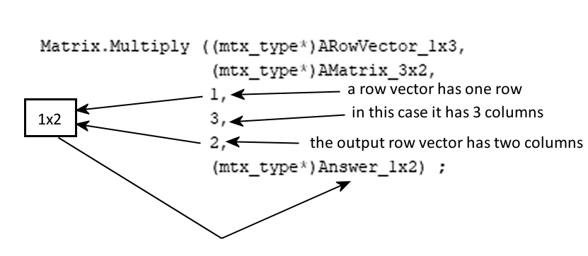
And I can now easily check my code to make sure that when the first parameter is a row vector, then the third parameter should be 1. Graphically:

There are lots of places in the code where I need to be careful about these sizes, so the diagram above helps me understand if I've got it right or not.

Part 4 Hidden Errors

Neural Networks on the Arduino Part 2: A start to changing the weights

In part one (read it before you read this) we saw how to create a neural network function which could run on an Arduino, but we missed out the most important part: how to train the network. Training here means changing the two matrices which connect the three vectors.

We train the network by back propagation of errors, so the network can reduce the errors and learn to get closer to the correct answer. It is called that because

1. The errors goes backwards from the output towards the input 
2. The errors are propagated into the network

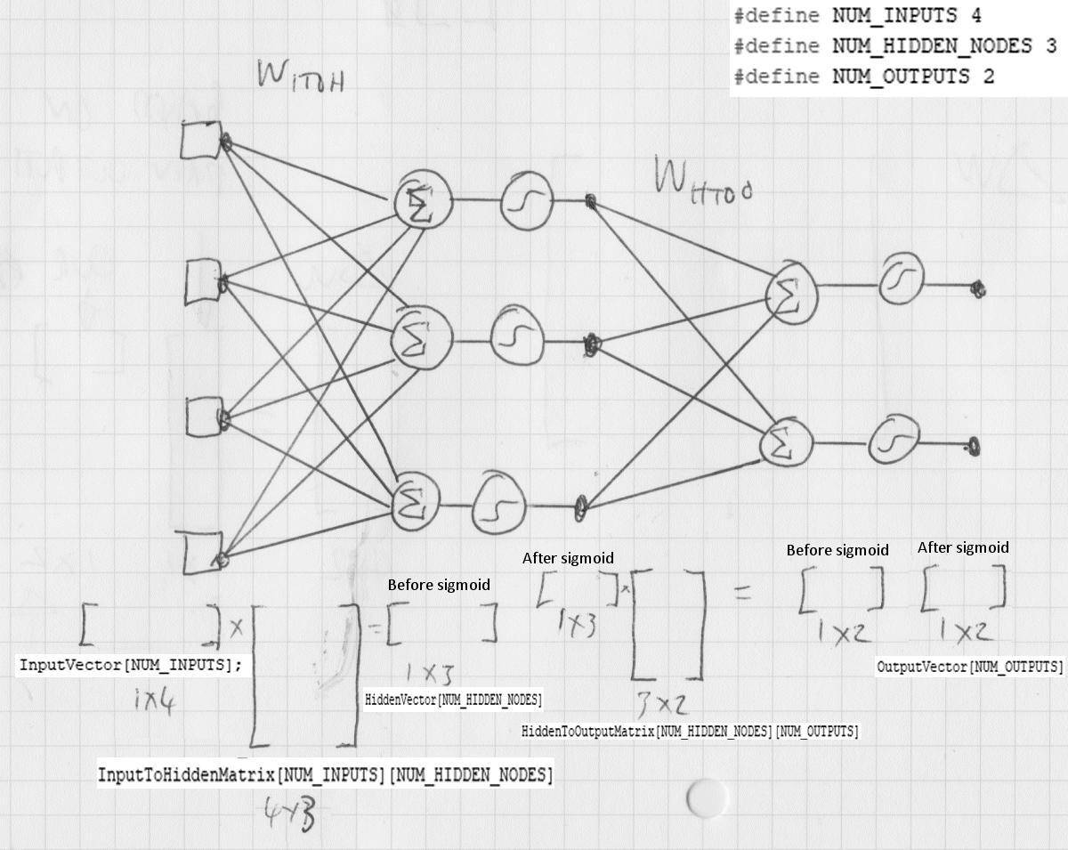
We'll be using the MatrixMath.h functions for the Arduino, here is a simple neural network and the matrices and vectors which represent it (remember weights are stored inside matrices):

Ok, so how to we change the weights to get the outputs closer to the targets? The best explanation I have found so far is in the book by Tariq Rashid...

... so I'll follow that, and translating from Python to Arduino C/C++. Here is the function from the book:

Here is the same thing in my blocky matrix type illustration

Stay with me. I had to draw these diagrams several times before I fully understood what I was doing.

The column vector  Oj (inputs to this layer (outputs from the previous layer)) multiplied by f (a row vector) create the matrix which are the changes to add (the deltas to apply) to the 3 x 2 matrix.

(a is the learning rate and is between 0 and 1 exclusive. A high learning rate (more than 0.5) may mean the network will never find a stable set of weights. A low learning rate may mean that it the training takes longer. In this Arduino version I've found that 0.1 is a good setting.)

The deltaW matrix is what we'll add to the original matrix to modify its weights.

HiddenToOutputMatrix, also obviously a 3 x 2. And we can follow a similar reasoning to the InputToHiddenMatrix, actually identical apart from the number of rows and columns. So shouldn't we put that inside a single function which can be called twice?

Look at the original diagram above, we can split it into two halves, and you can see that the architecture is the same, and only the sizes are different:

  First layer, input to hidden, 4 inputs and 3 outputs

Second layer, hidden to output, 3 inputs and 2 outputs

You can see that there are two layers.

As I said, this means is that it makes sense to have a single back propagation function which can be called twice instead of writing it all out twice. 

Note that in the Python implementation by Tariq Rashid the update of the weights by back propagation was done with a single "line" per layer. Here is one of those "lines":

self.who += self.lrate * 

            numpy.dot((output_errors*final_outputs*(1-final_outputs)),

            numpy.transpose(hidden_outputs))

who = weights-hidden-to-output. Why is there a "dot" in the above function? Well actually in Python this is the outer product. With the outer product two vectors produce a matrix, and in our case produces the matrix of changes to apply to the old matrix. For example:

It is always good to keep your feet on the ground when using matrices for neural networks, otherwise, if you're like me, you'll soon lose clarity about what the rows and columns are. 

In this case the number of rows in a matrix in a neural network layer are the number of inputs to the layer, and the number of columns in the matrix is the number of outputs. In images:

In the diagram above you can see a column vector and a row vector multiplied together to form a matrix. You do this using the outer product. Here it is in Arduino C:

// Outer product, from two vectors form a matrix
// C = A*B
// A is a column vector (vertical and has lots of rows)
// B is a row vector (horizontal and has lots of columns)
// C must have space for mRows and nColumns for this to work.
void OuterProduct(mtx_type* A, mtx_type* B, int mRows, int nColumns, mtx_type* C)
{
    int ra, cb;
    for (ra = 0; ra < mRows; ra++) {
        for(cb = 0; cb < nColumns; cb++)
        {
            // C[ra][cb] = C[ra][cb] + (A[ra] * B[cb]);
            C[(nColumns * ra) + cb] = A[ra] * B[cb];
        }
    }
} 

(The Arduino language is a sort of reduced C/C++ by the way, as far as I can understand. On the other hand the Arduino is so low-cost you can imagine putting Arduino neural networks to work anywhere.)

And here's Part 3: Details and tests of the matrix multiplication.